6. Mapping Lesson

6.1 Install WinSCP

6.1.1 Install WinSCP Tool

WinSCP is an open-source graphical SFTP client for Windows that supports the SSH and SCP protocols. It can securely copy files between local and remote computers. The tool can also directly edit files.

The installation steps for WinSCP are as follows:

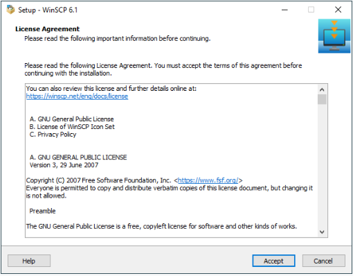
(1) Double-click the “WinSCP-5.15.3-Setup.exe” installation pack in the directory of this section. Click “Accept” to start installing.

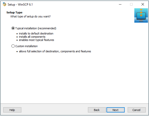
(2) Click “Next”.

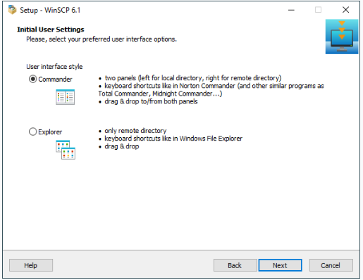
(3) Click “Next”.

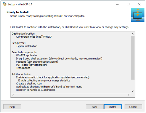
(4) Keep the default installation location and click “Install”.

(5) After waiting for a moment, a prompt window will appear indicating that the installation is complete. Click “Finish”.

(6) After the installation is completed, click to open it.

6.2 URDF Model

6.2.1 URDF Model Introduction

The Unified Robot Description Format (URDF) is an XML file format widely used in ROS (Robot Operating System) to comprehensively describe all components of a robot.

Robots are typically composed of multiple links and joints. A link is defined as a rigid object with certain physical properties, while a joint connects two links and constrains their relative motion.

By connecting links with joints and imposing motion restrictions, a kinematic model is formed. The URDF file specifies the relationships between joints and links, their inertial properties, geometric characteristics, and collision models.

6.2.2 Comparison between Xacro and URDF Models

The URDF model serves as a description file for simple robot models, offering a clear and easily understandable structure. However, when it comes to describing complex robot structures, using URDF alone can result in lengthy and unclear descriptions.

To address this limitation, the xacro model extends the capabilities of URDF while maintaining its core features. The xacro format provides a more advanced approach to describe robot structures. It greatly improves code reusability and helps avoid excessive description length.

For instance, when describing the two legs of a humanoid robot, the URDF model would require separate descriptions for each leg. On the other hand, the xacro model allows for describing a single leg and reusing that description for the other leg, resulting in a more concise and efficient representation.

6.2.3 Basic Syntax of URDF Model

• XML Basic Syntax

The URDF model is written using XML standard.

(1) Elements:

An element can be defined as desired using the following formula:

<element>

<element>

(2) Poperties:

Properties are included within elements to define characteristics and parameters. Please refer to the following formula to define an element with properties:

<element property_1="property value1" property_2="property value2">

<element>

(3) Comments:

Comments have no impact on the definition of other properties and elements. Please use the following formula to define a comment:

<!-- comment content -->

• Link

The Link element describes the visual and physical properties of the robot’s rigid component. The following tags are commonly used to define the motion of a link:

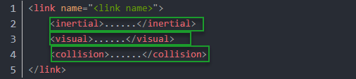
<visual>: Describe the appearance of the link, such as size, color and shape.

<inertial>: Describe the inertia parameters of the link, which will used in dynamics calculation.

<collision>: Describe the collision inertia property of the link.

Each tag contains the corresponding child tag. The functions of the tags are listed below.

Tag	Function
origin	Describe the pose of the link. It contains two parameters, including xyz and rpy. Xyz describes the pose of the link in the simulated map. Rpy describes the pose of the link in the simulated map.
mess	Describe the mess of the link
inertia	Describe the inertia of the link. As the inertia matrix is symmetrical, these six parameters need to be input, ixx, ixy, ixz, iyy, iyz and izz, as properties. These parameters can be calculated.
geometry	Describe the shape of the link. It uses mesh parameter to load texture file, and em[ploys filename parameters to load the path for texture file. It has three child tags, namely box, cylinder and sphere.
material	Describe the material of the link. The parameter name is the required filed. The tag color can be used to change the color and transparency of the link.

• Joint

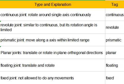
The “Joint” tag describes the kinematic and dynamic properties of the robot’s joints, including the joint’s range of motion, target positions, and speed limitations. In terms of motion style, joints can be categorized into six types.

The following tags will be used to write joint motion.

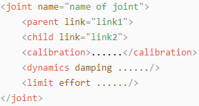
<parent_link>: Parent link

<child_link>: Child link

<calibration>: Calibrate the joint angle

<dynamics>: Describes some physical properties of motion

<limit>: Describes some limitations of the motion

The function of each tag is listed below. Each tag involves one or several child tags.

Tag	Function
origin	Describe the pose of the parent link. It involves two parameters, including xyz and rpy. Both xyz and rpy describe the pose of the link in simulated map.
axis	Control the child link to rotate around any axis of the parent link.
limit	The motion of the child link is constrained using the lower and upper properties, which define the limits of rotation for the child link. The effort properties restrict the allowable force range applied during rotation (values: positive and negative; units: N). The velocity properties confine the rotational speed, measured in meters per second (m/s).
mimic	Describe the relationship between joints.
safety_controller	Describes the parameters of the safety controller used for protecting the joint motion of the robot.

• Robot Tag

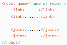
The complete top tags of a robot, including the <link> and <joint> tags, must be enclosed within the <robot> tag. The format is as follows:

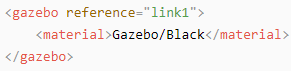
• gazebo Tag

This tag is used in conjunction with the Gazebo simulator. Within this tag, you can define simulation parameters and import Gazebo plugins, as well as specify Gazebo’s physical properties, and more.

• Write Simple URDF Model

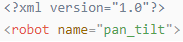
(1) Name the model of the robot

To start writing the URDF model, we need to set the name of the robot following this format: “<robot name=”robot model name”>”. Lastly, input “</robot>” at the end to represent that the model is written successfully.

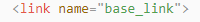
(2) Set links

① To write the first link and use indentation to indicate that it is part of the currently set model. Set the name of the link using the following format: <link name=”link name”>. Finally, conclude with “</link>” to indicate the successful completion of the link definition.

② Write the link description and use indentation to indicate that it is part of the currently set link, and conclude with “</visual>”.

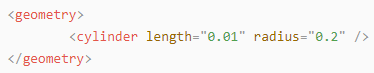
③ The “<geometry>” tag is employed to define the shape of a link. Once the description is complete, include “</geometry>”. Within the “<geometry>” tag, indentation is used to specify the detailed description of the link’s shape. The following example demonstrates a link with a cylindrical shape: “<cylinder length=”0.01” radius=”0.2”/>”. In this instance, “length=”0.01”” signifies a length of 0.01 meters for the link, while “radius=”0.2”” denotes a radius of 0.2 meters, resulting in a cylindrical shape.

④ The “<origin>” tag is utilized to specify the position of a link, with indentation used to indicate the detailed description of the link’s position. The following example demonstrates the position of a link: “<origin rpy=”0 0 0” xyz=”0 0 0” />”. In this example, “rpy” represents the roll, pitch, and yaw angles of the link, while “xyz” represents the coordinates of the link’s position. This particular example indicates that the link is positioned at the origin of the coordinate system.

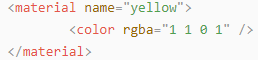
⑤ The “<material>” tag is used to define the visual appearance of a link, with indentation used to specify the detailed description of the link’s color. To start describing the color, include “<material>”, and end with “</material>” when the description is complete. The following example demonstrates setting a link color to yellow: “<color rgba=”1 1 0 1” />”. In this example, “rgba=”1 1 0 1”” represents the color threshold for achieving a yellow color.

(3) Set joint

① To write the first joint, use indentation to indicate that the joint belongs to the current model being set. Then, specify the name and type of the joint as follows: “<joint name=”joint name” type=”joint type”>”. Finally, include “</joint>” to indicate the completion of the joint definition.

Note: to learn about the type of the joint, please refer to “6.2.3 Basic Syntax of URDF Model -> Joint”.

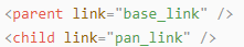
② Write the description section for the connection between the link and the joint. Use indentation to indicate that it is part of the currently defined joint. The parent parameter and child parameter should be set using the following format: “<parent link=”parent link”/>”, and “<child link=”child link” />”. With the parent link serving as the pivot, the joint rotates the child link.

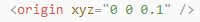
③ “<origin>” describes the position of the joint using indention. This example describes the position of the joint: “<origin xyz=”0 0 0.1” />”. xyz is the coordinate of the joint.

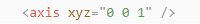
④ “<axis>” describes the position of the joint adopting indention. “<axis xyz=”0 0 1” />” describes one posture of a joint. xyz specifies the pose of the joint.

⑤ “<limit>” imposes restrictions on the joint using indention. The below picture The “<limit>” tag is used to restrict the motion of a joint, with indentation indicating the specific description of the joint angle limitations. The following example describes a joint with a maximum force limit of 300 Newtons, an upper limit of 3.14 radians, and a lower limit of -3.14 radians. The settings are defined as follows: “effort=’joint force (N)’, velocity=’joint motion speed’, lower=’lower limit in radians’, upper=’upper limit in radians’”.

⑥ “<dynamics>” describes the dynamics of the joint using indention. “<dynamics damping=”50” friction=”1” />” describes dynamics parameters of a joint.

The complete codes are as below.

6.3 ROS Robot URDF Model Instruction

6.3.1 Getting Ready

To grasp the URDF model, check out “6.3 ROS Robot URDF Model Introduction” for the key syntax. This part quickly breaks down the robot model code and its components.

6.3.2 Check Code of Robot Model

(1) Start the robot, and access the robot system desktop using VNC.

(2) Click-on to create a command-line terminal.

(3) Run the command and hit Enter to disable the app auto-start service.

~/.stop_ros.sh

(4) Execute the command and hit Enter key to navigate to the folder containing startup programs.

colcon_cd mentorpi_description

(5) Execute the command to navigate to the robot simulation model folder.

cd urdf

(6) Execute the command to access the robot simulation model folder.

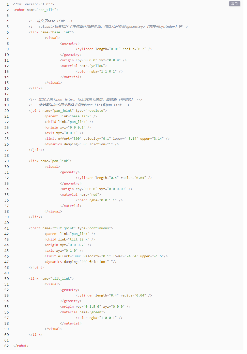
vim mentorpi.xacro

(7) Locate the code below:

Determine the current form of the robot by reading the machine variable to load the corresponding URDF model .

Multiple URDF models are called to compose a complete robot.

File Name	Device
inertial_matrix	Inertia matrix
mecanum	Mecanum urdf model
ack	Ackerman urdf model

After experiencing the Lidar game, you can activate the app service either by using a command or restarting the robot. If the app service is not activated, related app functions will be disabled. In the case of a robot restart, the app service will start automatically.

Click and enter the command. Press enter to start the app, and wait for the buzzer to beep.

Note

please enter the command in the system path, not in the Docker container.

sudo systemctl restart start_node.service

6.3.3 Brief Analysis of Robot’s Main Body Model

MentorPi has two types of chassis: Mecanum wheel chassis and Ackerman chassis. Here, we’ll focus on the Mecanum wheel chassis. Although the main model files for the Ackerman chassis are mostly the same, any differences will be explained later in this article.

Open a new command terminal. Enter the command to access the robot model file, which contains the description of each part of the robot model.

vim mecanum.xacro

<?xml version="1.0" ?>

<robot name="mecanum" xmlns:xacro="http://ros.org/wiki/xacro">

This is the beginning of the URDF file. It specifies the XML version and encoding, and defines a robot model named “mecanum”. The xmlns:xacro namespace is utilized here to generate URDF using Xacro macro definitions.

The following line of code defines a Xacro property named “black”, which means the black material.

<material name="black">

	<color rgba="0 0 0 1"/>

</material>

A joint called “imu_link” is defined with a type of “fixed”, indicating it’s a stationary joint. It connects the parent link “base_link” with the child link “imu_link”.

Then, the values of the joint’s origin and axis are defined.

<link name="imu_link"/>

  <joint name="imu_joint" type="fixed">

	<parent link="base_link"/>

	<child link="imu_link"/>

	<origin xyz="0 0 0" rpy="0 0 -1.57"/>

</joint\>

The link named “base_footprint” is defined as the robot’s chassis.

<link name="base_footprint"/>

<joint name="base_footprint_to_base_link" type="fixed">

<parent link="base_footprint"/>

<child link="base_link"/>

<origin xyz="0 0 0.07" rpy="0 0 0"/>

</joint>

The following code defines a link named “base_link”, including its inertial, visual, and collision properties.

The <inertial> section specifies the link’s inertial properties, like mass and inertia. It includes the <origin> tag, indicating the position and orientation of the inertial coordinate system relative to the link’s coordinate system. The <mass> tag denotes the link’s mass, and the <inertia> tag defines its moment of inertia about its principal axis.

The <visual> section determines the visual representation of the link. It includes the <origin> tag for the visualization coordinate system’s position and orientation relative to the link. The <geometry> tag defines the visual shape, here a grid, while the <mesh> tag specifies the file name of the mesh representing the link’s visual appearance. Lastly, the <material> tag specifies the color or texture. The “base_link.STL” defines the material.

The <collision> section specifies the link’s collision properties. It resembles the <visual> section but is for collision detection, not visualization. It includes the <origin> and <geometry> tags for defining position, direction, and shape of the collision representation.

In summary, this code defines a link in the robot model, detailing its inertial, visual, and collision properties. In simulations or visualizations, the mesh files specified in the <visual> and <collision> sections are utilized for visual representation and collision detection with other links.

<link name="base_link">

<inertial>

<origin rpy="0 0 0" xyz="7.82634169708696E-05 3.66518389137982E-05 0.0068167426737893"/>

<mass value="0.080358044299185"/>

<inertia ixx="9.92047502462735E-05" ixy="3.20099144678921E-08" ixz="1.15869166655817E-05" iyy="0.000292461515602123" iyz="-2.92890751882614E-08" izz="0.000367604260834833"/>

</inertial>

<visual>

<origin rpy="0 0 0" xyz="0 0 0"/>

<geometry>

<mesh filename="package://rosmentor_description/meshes/mecanum/base_link.STL"/>

</geometry>

<material name="">

<color rgba="1 1 1 1"/>

</material>

</visual>

<collision>

<origin rpy="0 0 0" xyz="0 0 0"/>

<geometry>

<mesh filename="package://rosmentor_description/meshes/mecanum/base_link.STL"/>

</geometry>

</collision>

</link>

The following code describes a link named “wheel_lf_Link”, which represents the left front wheel of the robot.

The <inertial> tag describes the inertial properties of the link, including its mass and moments of inertia. The mass of the link is set to 0.0378743634664218, and the values of its moments of inertia are specified. The <visual> tag defines the visual appearance of the link, including its geometry and color. The visual appearance of the link uses an STL mesh model located at “package://rosmentor_description/meshes/mecanum/wheel_lf_Link.STL”. The color is set to white with an RGBA value of 1 1 1 1, indicating a completely opaque white color.

The <collision> tag defines the collision properties of the link for collision detection. The collision model also uses an STL mesh model located at “package://rosmentor_description/meshes/mecanum/wheel_lf_Link.STL”

<link name="wheel_lf_Link">

<inertial>

<origin rpy="0 0 0" xyz="6.23194347770945E-05 -0.00574614971695361 2.98597149463314E-05"/>

<mass value="0.0378743634664218"/>

<inertia ixx="3.67678518315829E-06" ixy="-1.42189561270372E-09" ixz="-1.20320324868622E-08" iyy="5.81008995754212E-06" iyz="1.72329758812212E-09" izz="3.67939460898329E-06"/>

</inertial>

<visual>

<origin rpy="0 0 0" xyz="0 0 0"/>

<geometry>

<mesh filename="package://rosmentor_description/meshes/mecanum/wheel_lf_Link.STL"/>

</geometry>

<material name="">

<color rgba="1 1 1 1"/>

</material>

</visual>

<collision>

<origin rpy="0 0 0" xyz="0 0 0"/>

<geometry>

<mesh filename="package://rosmentor_description/meshes/mecanum/wheel_lf_Link.STL"/>

</geometry>

</collision>

</link>

The following is the description of the joint:

 <joint name="wheel_lf_Joint" type="continuous">
    <origin rpy="0 0 0" xyz="0.067052 0.07591 -0.018408"/>
    <parent link="base_link"/>
    <child link="wheel_lf_Link"/>
    <axis xyz="0.00012228 1 -4.0642E-05"/>
  </joint>

The above code defines a joint named “wheel_lf_Joint” for the left front wheel. The type of this joint is “continuous”, indicating that it is a continuously rotating joint used to describe a component that can rotate without limits, such as a wheel.

The <origin> tag specifies the position and orientation of the joint by xyz='0.067052 0.07591 -0.01'.

The parent and child links of the joint are specified using the <parent> and <child> tags, respectively. The parent link is “base_link”, and the child link is “wheel_lf_Link”, indicating that the joint connects the base link and the left front wheel link. The <axis> tag is used to define the rotation axis of the joint, with the direction specified by the xyz="0.00012228 1 -4.0642E-05" attribute.

This code describes a joint in a URDF file that connects the parent link “base_link” to the child link “wheel_lf_Link”. This joint describes the rotational connection of the left front wheel in the robot model, allowing it to rotate infinitely around the specified axis.

6.4 SLAM Mapping Principle

6.4.1 SLAM Introduction

SLAM stands for Simultaneous Localization and Mapping.

Localization involves determining the pose of a robot in a coordinate system. The origin of orientation of the coordinate system can be obtained from the first keyframe, existing global maps, landmarks or GPS data.

Mapping involves creating a map of the surrounding environment perceived by the robot. The basic geometric elements of the map are points. The main purpose of the map is for localization and navigation. Navigation can be divided into guidance and control. Guidance includes global planning and local planning, while control involves controlling the robot’s motion after the planning is done.

6.4.2 SLAM Mapping Principle

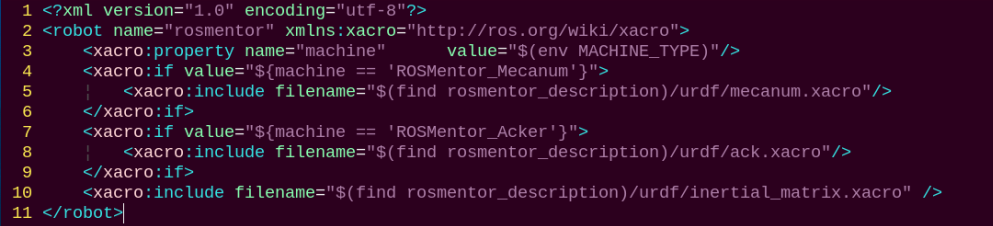
① Preprocessing: Optimizing the raw data from the radar point cloud, filtering out problematic data or performing filtering. Using laser as a signal source, pulses of laser emitted by the laser are directed at surrounding obstacles, causing scattering.

Some of the light waves will reflect back to the receiver of the lidar, and then, according to the principle of laser ranging, the distance from the lidar to the target point can be obtained.

Regarding point clouds: In simple terms, the surrounding environment information obtained by lidar is called a point cloud. It reflects a portion of what the ‘eyes’ of the robot can see in the environment where it is located. The object information collected presents a series of scattered, accurate angle, and distance information.

② Matching: Matching the point cloud data of the current local environment with the established map to find the corresponding position.

③ Map Fusion: Integrating new round data from the lidar into the original map, ultimately completing the map update.

6.4.3 Notes

(1) Begin the mapping process by positioning the robot in front of a straight wall or within an enclosed box. This enhances the Lidar’s capacity to capture a higher density of scanning points.

(2) Initiate a 360-degree scan of the environment using the Lidar to ensure a comprehensive survey of the surroundings. This step is crucial to guarantee the accuracy and completeness of the resulting map.

(3) For larger areas, it’s recommended to complete a full mapping loop before focusing on scanning smaller environmental details. This approach enhances the overall efficiency and precision of the mapping process.

6.4.4 Judge Mapping Result

Finally, assess the robot’s navigation process against the following criteria once the mapping is complete:

(1) Ensure that the edges of obstacles within the map are distinctly defined.

(2) Check for any disparities between the map and the actual environment, such as the presence of closed loops or inconsistencies.

(3) Verify the absence of gray areas within the robot’s motion area, indicating areas that haven’t been adequately scanned.

(4) Confirm that the map doesn’t incorporate obstacles that won’t exist during subsequent localization.

(5) Validate the map’s coverage of the entire extent of the robot’s motion area.

6.5 slam_toolbox Mapping Algorithm

6.5.1 Algorithm Definition

Slam Toolbox software package combines information from laser rangefinders in the form of LaserScan messages and performs TF transformation from odom-> base link to create a two-dimensional map of space. This software package allows for fully serialized reloadable data and pose graphs of SLAM maps, used for continuous mapping, localization, merging, or other operations. It allows Slam Toolbox to operate in synchronous (i.e., processing all valid sensor measurements regardless of delay) and asynchronous (i.e., processing valid sensor measurements whenever possible) modes.

ROS replaces functionalities like gmapping, cartographer, karto, and hector, providing comprehensive SLAM functionality built upon the powerful scan matcher at the core of Karto, widely used and accelerated for this package. It also introduces a new optimization plugin based on Google Ceres. Additionally, it introduces a new localization method called ‘elastic pose-graph localization,’ which takes measured sliding windows and adds them to the graph for optimization and refinement. This allows for tracking changes in local features of the environment instead of considering them as biases, and removes these redundant nodes when leaving an area without affecting the long-term map.

Slam Toolbox is a suite of tools for 2D Slam, including:

● Mapping, saving map pgm files

● Map refinement, remapping, or continuing mapping on saved maps

● Long-term mapping: loading saved maps to continue mapping while removing irrelevant information from new laser point clouds

● Optimizing positioning mode on existing maps. Localization mode can also be run without mapping using the ‘laser odometry’ mode

● Synchronous, asynchronous mapping

● Dynamic map merging

● Plugin-based optimization solver, with a new optimization plugin based on Google Ceres

● Interactive RVIZ plugin

● RVIZ graphical manipulation tools for manipulating nodes and connections during mapping

● Map serialization and lossless data storage.

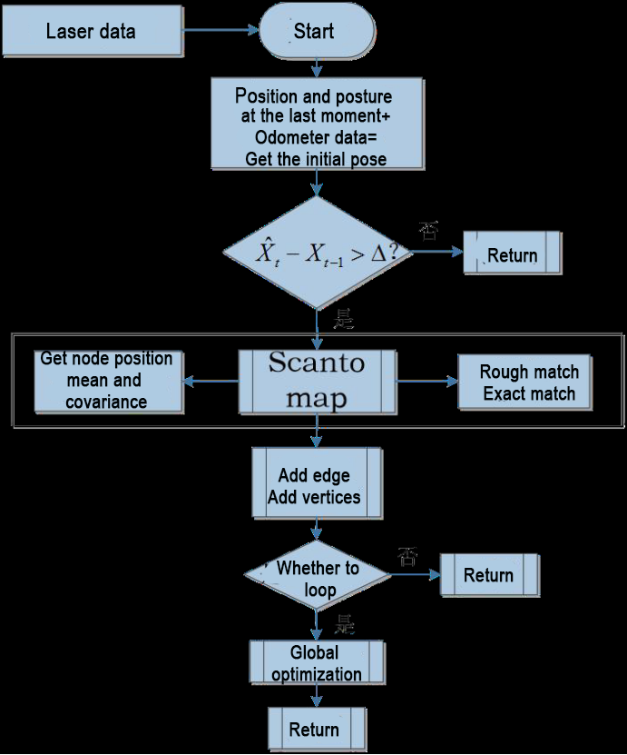
From the above diagram, it can be seen that the process is relatively straightforward. The traditional soft real-time operation mechanism of slam involves processing each frame of data upon entry and then returning.

Relevant source code and WIKI links for KartoSLAM:

• KartoSLAM ROS Wiki: http://wiki.ros.org/slam_karto

• slam_karto software package: https://github.com/ros-perception/slam_karto

• open_karto open-source algorithm: https://github.com/ros-perception/open_karto

6.5.2 Mapping Operation Steps

ROS2 mapping and navigation utilize virtual machine connectivity to enable mapping and navigation with the robot on the same local network.

• Install Virtual Machine Software and Import the Virtual Machine

(1) Unzip the provided installation files, then click on the installation file to proceed with the installation.

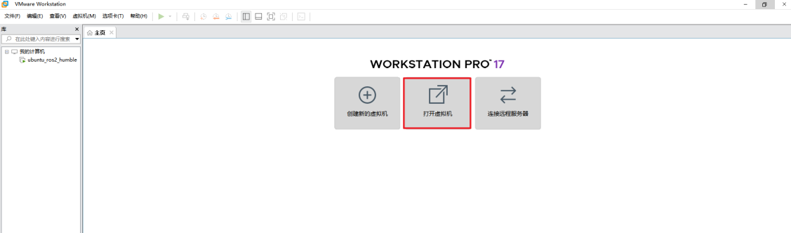
(2) Click on to open the virtual machine.

(3) Enter the virtual machine interface and click on “Open Virtual Machine”.

(4) Select the image file provided in the tutorial and import it. For specific instructions, please refer to the lesson “5. Depth Camera Basic Lesson/Test and Configure ROS2”.

(5) After the import is completed, follow the prompts to complete the installation process.

• Copy Robot Files to the Virtual Machine

(1) Export files from the robot

① Start the robot, and access the robot system desktop using VNC.

② Click-on to open the ROS2 command-line terminal.

③ Execute the command to disable the app auto-start service.

~/.stop_ros.sh

④ Enter the command to navigate to the ros2_ws/src/ directory:

cd ros2_ws/src/

⑤ Enter the command to package the three files ‘navigation’, ‘slam’, and ‘simulations’ into a compressed file:

zip -r src.zip navigation slam simulations

⑥ Enter the command to move the compressed file to the shared directory:

mv src.zip /home/ubuntu/shared

⑦ Run the command and return to ros2_ws directory:

cd ..

⑧ Enter the command to view the .typerc file in this directory:

ls -a

⑨ Enter the command to move the .typerc file to the shared directory:

cp .typerc /home/ubuntu/shared

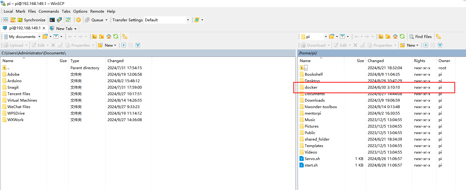
⑩ Click-on to open the file directory, then navigate to the home/docker/tmp directory:

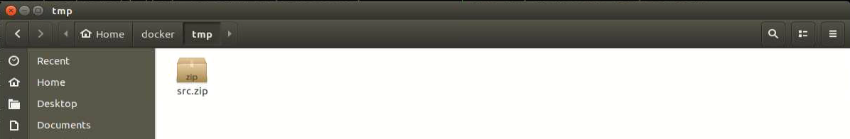
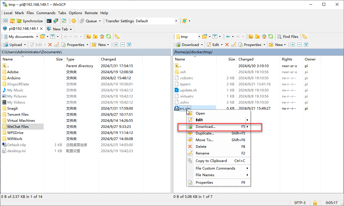
⑪ Use the shortcut ‘Ctrl + H’ to show the hidden .typerc file:

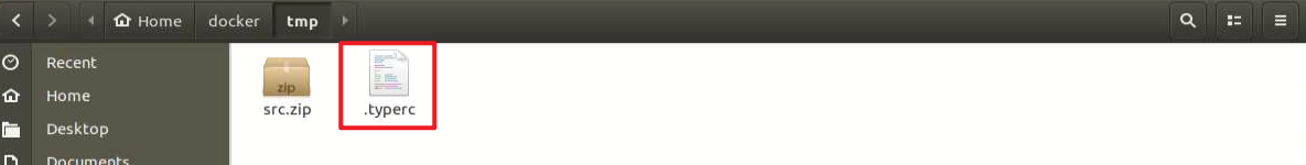
⑫ Refer to the instruction in “Install WinSCP” to install and open the WinSCP tool.

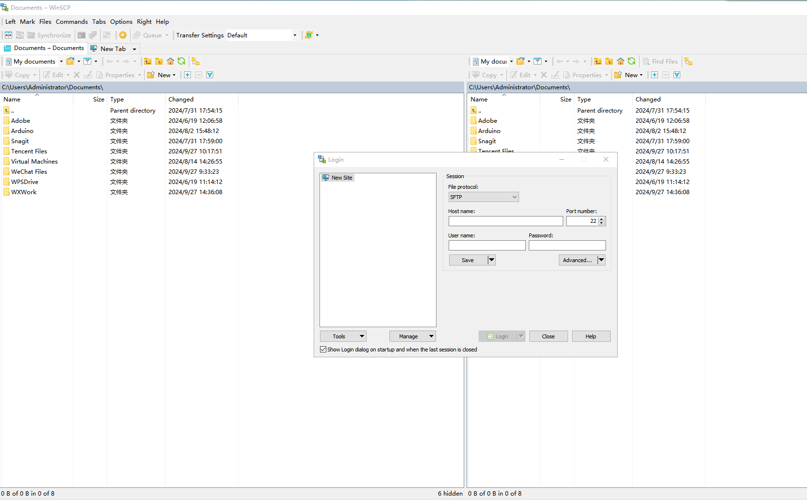
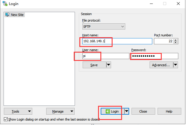
⑬ Enter the IP address of Raspberry Pi “192.168.149.1”, username “pi”, and password “raspberrypi”. Then click “Login”.

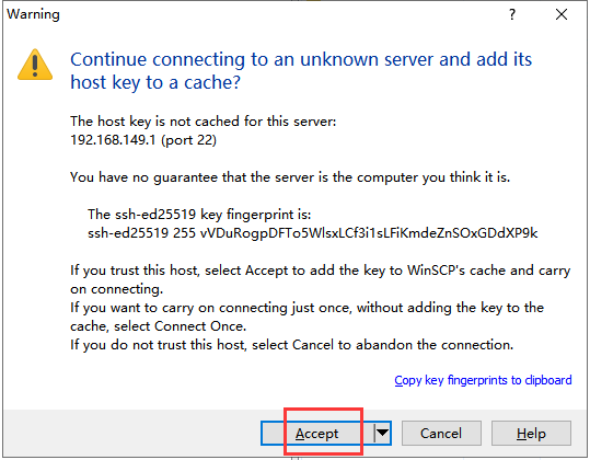
⑭ Click “Accept” on the pop-up window that appears.

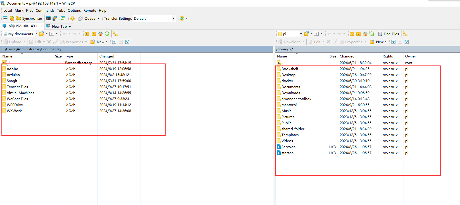
⑮ The left side shows the directory of your computer, and the right side shows the root directory of Raspberry Pi.

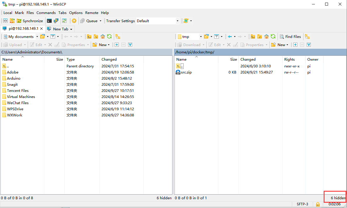
⑯ Select the folder “docker->tmp” and open the shared folder with Docker.

⑰ In the bottom right corner of WinSCP, there is a number indicating the number of hidden files. Double-click on it to display hidden files.

⑱ Select the “src” folder and right-click to choose “Download”.

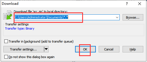
⑲ Select the path where you want to save the file and click “OK”.

⑳ Follow step ⑱ to save the .typerc file.

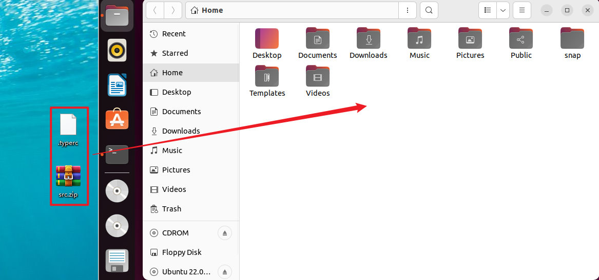
(2) Import files into the virtual machine

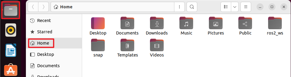
① Click-on to navigate to the home directory.

② Drag and drop the .typerc and src.zip files from the computer desktop into the virtual machine:

5.2.3 Create and Compile the Workspace

(1) Click-on to start the virtual machine command-line terminal.

(2) Enter the command to create the ros2_ws/src directory:

mkdir -p ros2_ws/src

(3) Extract the file “src.zip” to the directory “home/ubuntu”.

unzip src.zip

(4) Move the simulations, slam, and navigation files to the ros2_ws/src directory:

mv simulations slam navigation /home/ubuntu/ros2_ws/src/

(5) Move the .typerc file to the ros2_ws directory:

mv .typerc ros2_ws/

(6) Navigate to the ros2_ws directory:

cd ros2_ws/

(7) Enter the command to check if .typerc has been moved to the ros2_ws directory:

ls -a

(8) Input the following command to compile the workspace:

colcon build

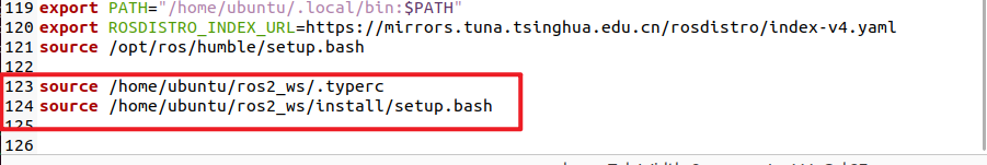
(9) Change the .bashrc file, and input the following command:

gedit ~/.bashrc

Copy the content below to the file .bashrc.

source /home/ubuntu/ros2_ws/.typerc
source /home/ubuntu/ros2_ws/install/setup.bash

(10) After finishing writing, use the shortcut Ctrl + S or click the Save button in the upper right corner to save and exit.

(11) Run the command below to refresh the environment configuration.

source ~/.bashrc

• Set the Robot to LAN Mode

(1) Click-on to open the command line terminal.

(2) Enter the command to open the WiFi configuration file.

vim hiwonder-toolbox/wifi_conf.py

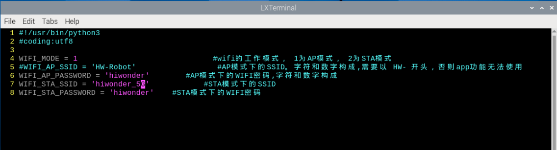
(3) Press “i” key to enter the editing mode. Change the WiFi configuration file to LAN mode, and modify your own WiFi name and password.

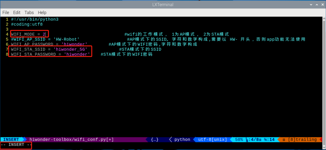
(4) After finishing writing, press “Esc” and enter the command to save and exit.

:wq

(5) Enter the command to restart the network, or reboot the system. It is recommended to reboot the system.

sudo systemctl restart wifi.service

(6) Refer to “Getting Ready -> APP Control” to obtain the robot’s LAN IP address through the app connection.

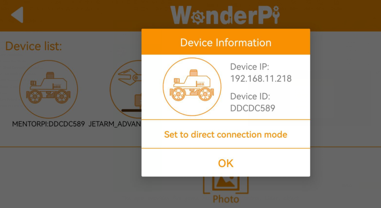
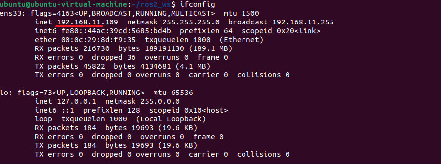
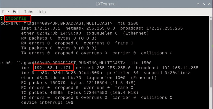
(7) It is important to note that the virtual machine and the robot are connected to the same LAN, and their IP addresses should be within the same subnet:

① Virtual Machine:

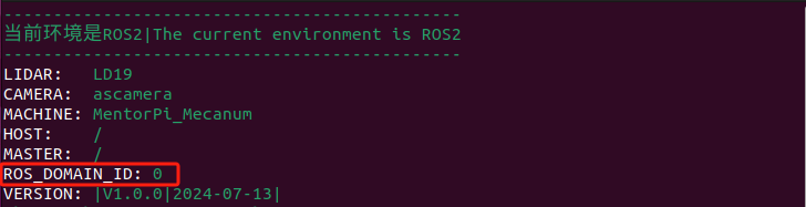
② Robot:

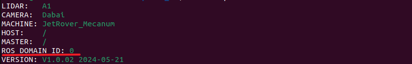
(8) After rebooting, click on to open the robot’s ROS2 command line terminal. You will notice that the ROS_DOMAIN_ID is 0, which is the same as on the virtual machine.

① Robot:

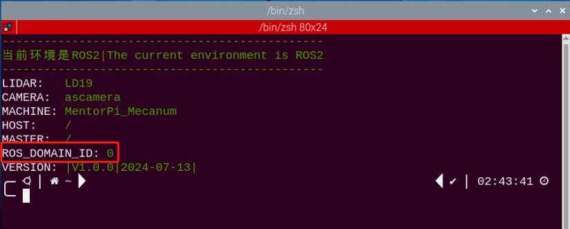
② Virtual Machine:

6.5.3 slam Mapping Instructions

• Robot operations

(1) Click-on to open the command-line terminal.

(2) Execute the following command to disable the app auto-start service.

~/.stop_ros.sh

(3) Run the command to initiate mapping:

ros2 launch slam slam.launch.py

• Virtual Machine instructions

(1) Click-on to open the command line terminal of the virtual machine system.

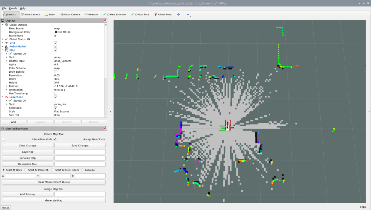
(2) Enter the command to open the RViz tool and display the mapping results.

ros2 launch slam rviz_slam.launch.py

• Enable keyboard control

(1) Click-on to open the command-line terminal.

(2) Enter the command to start the keyboard control node, and press “Enter”.

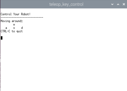
ros2 launch peripherals teleop_key_control.launch.py

If you see the prompt as shown in the following image, it means the keyboard control service has been successfully started.

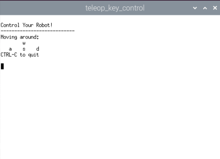
(3) Control the robot to move in the current space to build a more complete map. The table below lists the keyboard keys available for controlling robot movement and their corresponding functions:

Key	Robot Action
W	Short press to switch to forward state and continuously move forward
S	Short press to switch to backward state and continuously move backward
A	Long press to interrupt the forward or backward state and turn left
D	Long press to interrupt the forward or backward state and turn right

(4) When controlling the robot’s movement with the keyboard to map, it’s advisable to reduce the robot’s movement speed appropriately. The slower the robot’s speed, the smaller the odometry relative error, leading to better mapping results. As the robot moves, the map displayed in RVIZ will continuously expand until the entire environment scene’s map construction is completed.

6.5.4 Save Map

(1) Click-on to open the command-line terminal.

(2) Run the following command to save the map.

cd ~/ros2_ws/src/slam/maps && ros2 run nav2_map_server map_saver_cli -f "map_01" --ros-args -p map_subscribe_transient_local:=true

(3) If you want to exit the game, press “Ctrl+C” in the terminal interface.

After experiencing the game, you can enable the app service through commands or by restarting the robot. If the app is not enabled, the related app functions will not work. If the robot is restarted, the app will be automatically enabled.

Click and enter the command. Press enter to start the app, and wait for the buzzer to beep.

Note

please enter the command in the system path, not in the Docker container.

sudo systemctl restart start_node.service

6.5.5 Effect Optimization

If you desire a more precise mapping outcome, optimizing the odometry can be beneficial. Mapping with the robot requires the use of odometry, which in turn relies on the IMU.

The robot itself comes with pre-calibrated IMU data loaded, enabling it to perform mapping and navigation functions effectively. However, calibrating the IMU can still enhance accuracy further. The calibration method and steps for the IMU can be found in the “3. Motion Control Lesson -> 3.3 IMU, Linear Velocity and Angular Velocity Calibration” section.

6.5.6 Parameter Explanation

The parameter file can be found in the “ros2_ws\src\slam\config\slam.yaml” directory.

For more detailed information about the parameters, please refer to the official documentation: https://wiki.ros.org/slam_toolbox

6.5.7 Launch File Analysis

The launch file is located at:/home/ubuntu/ros2_ws/src/slam/launch/slam.launch.py

• Import Library

The launch library can be explored in detail in the official ROS documentation:

https://docs.ros.org/en/humble/How-To-Guides/Launching-composable-nodes.html

import os
from ament_index_python.packages import get_package_share_directory

from launch_ros.actions import PushRosNamespace
from launch import LaunchDescription, LaunchService
from launch.substitutions import LaunchConfiguration
from launch.launch_description_sources import PythonLaunchDescriptionSource
from launch.actions import DeclareLaunchArgument, IncludeLaunchDescription, GroupAction, OpaqueFunction, TimerAction

• Set the Storage Path

Use the “get_package_share_directory” function to obtain the path of the slam package.

    if compiled == 'True':
        slam_package_path = get_package_share_directory('slam')
    else:
        slam_package_path = '/home/ubuntu/ros2_ws/src/slam'

• Initiate Other Launch File

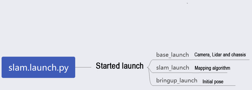
    base_launch = IncludeLaunchDescription(
        PythonLaunchDescriptionSource(
            os.path.join(slam_package_path, 'launch/include/robot.launch.py')),
        launch_arguments={
            'sim': sim,
            'master_name': master_name,
            'robot_name': robot_name
        }.items(),
    )

    slam_launch = IncludeLaunchDescription(
        PythonLaunchDescriptionSource(
            os.path.join(slam_package_path, 'launch/include/slam_base.launch.py')),
        launch_arguments={
            'use_sim_time': use_sim_time,
            'map_frame': map_frame,
            'odom_frame': odom_frame,
            'base_frame': base_frame,
            'scan_topic': f'{frame_prefix}scan_raw',  # Using scan_raw topic
            'enable_save': enable_save
        }.items(),
    )

    if slam_method == 'slam_toolbox':
        bringup_launch = GroupAction(
            actions=[
                PushRosNamespace(robot_name),
                base_launch,
                TimerAction(
                    period=10.0,
                    actions=[slam_launch],
                ),
            ]
        )

base_launch: Launch for hardware initialization

slam_launch: Launch for basic mapping

bringup_launch: Launch for initial pose setup

6.6 RTAB-VSLAM 3D Mapping

6.6.1 RTAB-VSLAM Description

RTAB-VSLAM is a appearance-based real-time 3D mapping system, it’s an open-source library that achieves loop closure detection through memory management methods. It limits the size of the map to ensure that loop closure detection is always processed within a fixed time limit, thus meeting the requirements for long-term and large-scale environment online mapping.

6.6.2 RTAB-VSLAM Working Principle

RTAB-VSLAM 3D mapping employs feature mapping, offering the advantage of rich feature points in general scenes, good scene adaptability, and the ability to use feature points for localization. However, it has drawbacks, such as a time-consuming feature point calculation method, limited information usage leading to loss of image details, diminished effectiveness in weak-texture areas, and susceptibility to feature point matching errors, impacting results significantly.

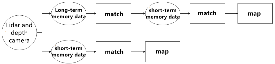
After extracting features from images, the algorithm proceeds to match features at different timestamps, leading to loop detection. Upon completion of matching, data is categorized into long-term memory and short-term memory. Long-term memory data is utilized for matching future data, while short-term memory data is employed for matching current time-continuous data.

During the operation of the RTAB-VSLAM algorithm, it initially uses short-term memory data to update positioning points and build maps. As data from a specific future timestamp matches long-term memory data, the corresponding long-term memory data is integrated into short-term memory data for updating positioning and map construction.

RTAB-VSLAM software package link: https://github.com/introlab/rtabmap

6.6.3 RTAB-VSLAM 3D Mapping Instructions

• Robot Operations

(1) Click on on the system desktop to open the command-line terminal.

(2) Run the command to disable the app auto-start service:

~/.stop_ros.sh

(3) Execute the command to start mapping:

ros2 launch slam rtabmap_slam.launch.py

• Virtual Machine Operation

(1) Click-on to open the command-line terminal.

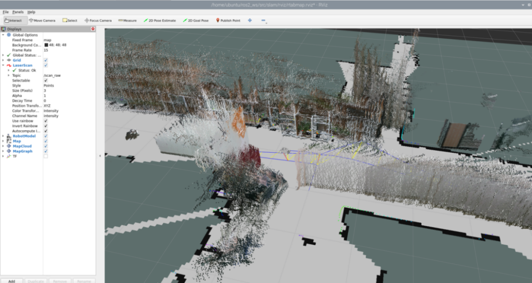
(2) Enter the command to open the RViz tool and display the mapping effect:

ros2 launch slam rviz_rtabmap.launch.py

• Enable Keyboard Control

(1) Click-on to open the command-line terminal.

(2) Enter the command to start the keyboard control node, and press “Enter”.

ros2 launch peripherals teleop_key_control.launch.py

If you encounter the prompt as shown in the figure below, it means that the keyboard control service has been successfully activated.

(3) Control the robot to move in the current space to build a more complete map. The table below shows the keyboard keys available for controlling robot movement and their corresponding functions:

Key	Robot Action
W	Short press to switch to the forward state and continuously move forward
S	Short press to switch to the backward state and continuously move backward
A	Long press to interrupt the forward or backward state and turn left
D	Long press to interrupt the forward or backward state and turn right

When controlling the robot’s movement for mapping using the keyboard, it’s advisable to appropriately reduce the robot’s movement speed. The smaller the robot’s running speed, the smaller the relative error of the odometry, resulting in a better mapping effect. As the robot moves, the map displayed in RVIZ will continuously expand until the entire environmental scene’s map construction is completed.

• Map Saving

After mapping is completed, you can use the shortcut “Ctrl+C” in each command-line terminal window to close the currently running program.

After experiencing the game, you can enable the app service through commands or by restarting the robot. If the app is not enabled, the related app functions will not work. If the robot is restarted, the app will be automatically enabled.

Click and enter the command. Press enter to start the app, and wait for the buzzer to beep.

Note

please enter the command in the system path, not in the Docker container.

sudo systemctl restart start_node.service

Note

For 3D mapping, there’s no need to manually save the map. When you use “Ctrl+C” to close the mapping command, the map will be automatically saved.

• Launch File Analysis

The launch file is located at: /home/ubuntu/ros2_ws/src/slam/launch/rtabmap_slam.launch.py

(1) Import Library:

You can refer to the ROS official documentation for detailed analysis of the launch library:

“https://docs.ros.org/en/humble/How-To-Guides/Launching-composable-nodes.html”

import os
from ament_index_python.packages import get_package_share_directory
from launch_ros.actions import PushRosNamespace
from launch import LaunchDescription
from launch.substitutions import LaunchConfiguration
from launch.launch_description_sources import PythonLaunchDescriptionSource
from launch.actions import DeclareLaunchArgument, IncludeLaunchDescription, GroupAction, OpaqueFunction, TimerAction

(2) Set the Storage Path

Use “get_package_share_directory” to obtain the path of the slam package.

    if compiled == 'True':
        slam_package_path = get_package_share_directory('slam')
    else:
        slam_package_path = '/home/ubuntu/ros2_ws/src/slam'

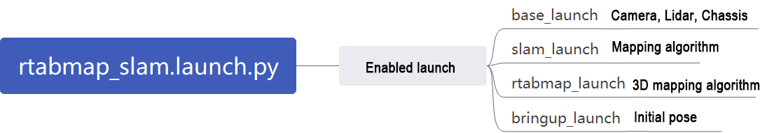
(3) Initiate Other Launch File

    base_launch = IncludeLaunchDescription(
        PythonLaunchDescriptionSource(
            os.path.join(slam_package_path, 'launch/include/robot.launch.py')),
        launch_arguments={
            'sim': sim,
            'master_name': master_name,
            'robot_name': robot_name,
            'action_name': 'horizontal',
        }.items(),
    )    
    

    rtabmap_launch = IncludeLaunchDescription(
        PythonLaunchDescriptionSource(
            os.path.join(slam_package_path, 'launch/include/rtabmap.launch.py')),
        launch_arguments={
            'use_sim_time': use_sim_time, 
        }.items(),
    )
    
    bringup_launch = GroupAction(
     actions=[
         PushRosNamespace(robot_name),
         base_launch,
         TimerAction(
             period=10.0, 
             actions=[rtabmap_launch],
         ),
      ]
    )

base_launch: Launch for hardware initialization

slam_launch: Basic mapping launch

rtabmap_launch: RTAB mapping launch

bringup_launch: Initial pose launch